Machine learning for neuroimaging

Information
The estimated time to complete this training module is 4h.
The prerequisites to take this module are:
- installation module
- introduction to python for data analysis module
- introduction to machine learning module
Recommended but not mandatory :
- fmri connectivity module
- fmri parcellation module
If you have any questions regarding the module content please ask them in the relevant module channel on the school Discord server. If you do not have access to the server and would like to join, please send us an email at school [dot] brainhack [at] gmail [dot] com.
Follow up with your local TA(s) to validate you completed the exercises correctly.
Resources
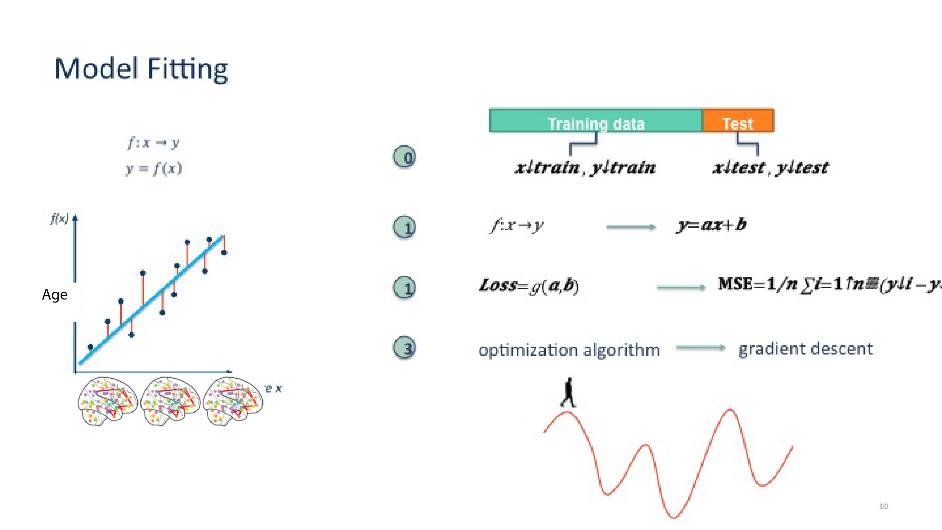
This module was presented by Jacob Vogel during the QLSC 612 course in 2020, the slides are available here.
The video of the presentation is available below (2h13):
If you need to resfresh some machine learning concepts before this tutorial, you can find the link to the slides from the introduction to machine learning here: https://github.com/neurodatascience/course-materials-2020/blob/master/lectures/14-may/03-intro-to-machine-learning/IntroML_BrainHackSchool.pdf
Exercise
- Download the jupyter notebook (save raw version), or start a new jupyter notebook
- Watch the video and test the code yourself
Using the same dataset:
Tweak the pipeline in the tutorial, by applying PCA , keeping 90% of the variance, instead of SelectPercentile to reduce the dimensionality of features (feature selection). Refer to scikit-learn documentation. https://scikit-learn.org/stable/modules/generated/sklearn.decomposition.PCA.html
 model = Pipeline([
 ('feature_selection',SelectPercentile(f_regression,percentile=20)),
 ('prediction', l_svr)
               ])
Implement cross-validation, but this time changing to leave-one-out. Here is to give an idea as to where changes need to be made in the code.
# First we create 10 splits of the data
skf = KFold(n_splits=10, shuffle=True, random_state=123)
What are the features we are using in this model? What are the numbers representing the shape of the time series (168, 64), the shape of the connectivity matrix (64 x 64), and of the feature matrix (155, 2016)?
Using the performance of the different polynomial fit (MSE) for train and test error, try to explain why increasing complexity of models does not necessarily lead to a better model.
Remember we talked about regularization in the introduction to machine learning? Variance of model estimation increases when there are more features than samples. This is especially relevant when we have > 2000 features ! Apply a penalty to the SVR model. Refer to the documentation https://scikit-learn.org/stable/modules/generated/sklearn.svm.LinearSVR.html.
Bonus: Try to run a SVC with a linear kernel to classify Children and Adults labels (pheno[‘Child_Adult’]). What can you say about the performance of your model ?
- Follow up with your local TA(s) to validate you completed the exercises correctly.
- 🎉 🎉 🎉 you completed this training module! 🎉 🎉 🎉
More resources
- Dataset used : https://openneuro.org/datasets/ds000228/versions/1.0.0
- scikit-learn documentation : https://scikit-learn.org/stable/
- Nilearn plotting functions : https://nilearn.github.io/stable/plotting/index.html
- Python Data Science Handbook’s chapter on machine learning by Jake VanderPlas is an excellent resource, although not openly available online