fMRI Stats Exploration

Deliverables

• Project Proposal
• Project Presentation
• GitHub repository
• Reproduction steps
• Analysis notebook
• Resulting figures

Project description

The project represents my own personal first experience handling neuroimaging data.

Coming from a Deep Learning background, this project represents the type of analysis I would undertake in order to get a better feel of what exactly am I trying to train models on.

One extremely important element of training DL models is to make sure that the distribution of the data is well-suited for modeling. This generally means having the data take shape of a standard or uniform distribution with values concentrated between -1 and 1. I observed that original fMRI data does not necessarily fit those criteria and that the distribution between subjects can also vary substantially (Figure a). This distribution looks quite unnatural to fit back into one of the mentioned distributions, however, Figure q demonstrates that it is possible.

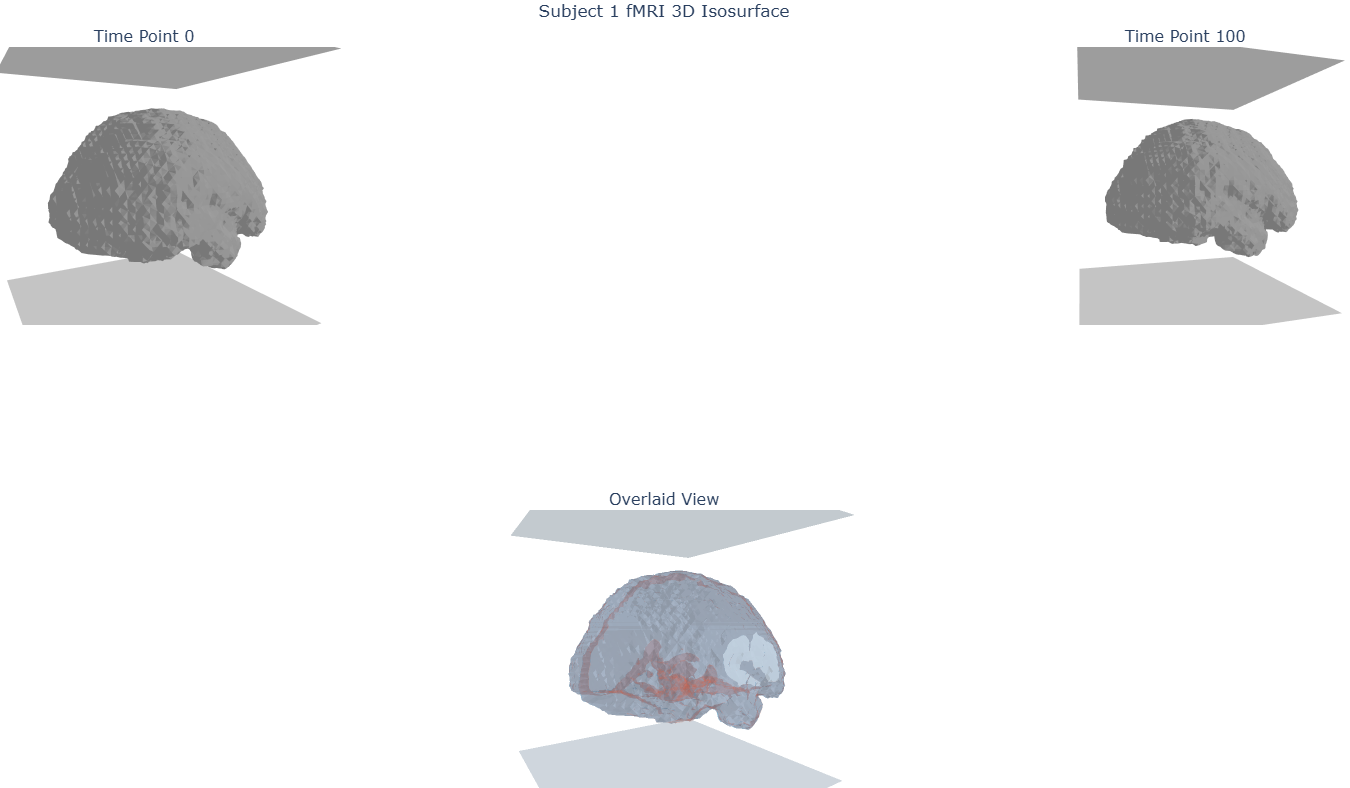
I then wanted to get a better feel of what does that original data looks like in 3D (Figure b & c) before taking a look at how does the data vary across time. In Figure d, I take a look at the overlapping differences between two collected timepoints in order to get a better feel of what are supposedly movements by the subject in the scanner. In Figure e, I generalize that to the entire series of timepoints to get a feel of where variance is most present, which we notice to be at the edges of the brain, seeming to correlate to those same brain movements (Note: I did not account for the fact that the data is in its original distribution at that point in time which could have biased my observations).

Next, one important element that I wanted to get more understanding of is the various transformations applied on top of the raw fMRI data. Indeed, AI practitioners are often wary of transformations being applied to data prior to feeding it to AI models as those transformations can greatly impact the model’s ability to learn something valuable. I thus took a closer at the applications of confounds. I first extracted the data that gets added to the signal as a result of applying those very confounds and visualized it in 3D (Figure f & g). It very much looks like noise though with a little bit of a pattern of lower values around the edges of the brain.

I then moved on to taking a closer look at the 3D difference between the original data (Figure a), the data with confounds applied (Figure h) and the data with confounds and a threshold applied (as demonstrated in the course) (Figure i). Visibly, applying the confounds looks like it is simply getting rid of the data where no brain data is ever collected, while the thresholding observed in class is more agressive and appears to chunk out a lot of the data (some seemingly relevant? not sure, too new at this hehe).

I then went back to observing variance across time as done in Figure e but this time with the confounds and threshold applied (Figure j). In that visualization we observe that the largest variance no longer only occurs at the edge of the brain but also where the white matter is supposedly located, seeming to indicate that the head movement was somewhat corrected (Also note by dragging the cursor that the variance is generally much lower in general: 2 vs 3 orders of magnitude).

At that point I wanted to quickly go back to connectivity matrices to see the effects of the confounds (Figure k applied, Figure l not applied). Because while the application of confounds do not amount to much information when visualizing in 3D, they do appear very important when converting to atlases and computing connectivity matrices.

From then on, I somewhat concluded that the intuition that I was building in the original 3D space was not fully transferable to the parcel space.

I thus moved on to the Algonauts data and started with taking a look at their 3D -> parcel space transformation, orchestrated through the Schaefer 2018 Atlas [3] (Figure m).

I then went on to selecting a given subject and picking a given scene (Figure n) and taking a look at the resulting fMRI data projected back into 3D (Figure o & p). This looks completely different from what I had been working on so far. The distribution of the data looks ameneable to train models with (Figure p & q) and the different brain regions have clear differences in activation values. A correlation matrix computed on that series of data (Figure q) seals the deal with clear positive and negative correlation between brain regions which is to be expected.

On my end, a simple question remains unanswered: how did we go from such a noisy signal to such a clear cut signal? It seems like decades of work from the scientific community has gone into those transformations, and I look forward to learning more about those as I get more familiar with fMRI brain data :)

Data Used

• Nilearn’s brain development dataset [1]
• Algonauts 2025 dataset [2]

Tools Used

Development

• Visual Studio Code
• Python
• Jupyter notebooks
• Git/GitHub

Containerization

• Docker
• Dev Containers
• Docker Hub

Plotting

• Matplotlib
• Bokeh
• Plotly

Neuroimaging

• Nilearn
• Nibabel

References

[1] Hilary Richardson, Grace Lisandrelli, Alexa Riobueno-Naylor, and Rebecca Saxe. Development of the social brain from age three to twelve years. Nature communications, 9(1):1–12, 2018.

[2] Gifford, Alessandro T., et al. “The Algonauts Project 2025 Challenge: How the Human Brain Makes Sense of Multimodal Movies.” arXiv preprint arXiv:2501.00504 (2024).

[3] Alexander Schaefer, Ru Kong, Evan M Gordon, Timothy O Laumann, Xi-Nian Zuo, Avram J Holmes, Simon B Eickhoff, and B T Thomas Yeo. Local-Global Parcellation of the Human Cerebral Cortex from Intrinsic Functional Connectivity MRI. Cerebral Cortex, 28(9):3095–3114, 07 2017